
Research about SQL Database
Here is some research about SQL Database.
Ref:
-
Index: https://viblo.asia/p/b-tree-indexes-database-indexing-complete-guide-oW4oeeokLml
-
Storage: https://viblo.asia/p/database-storage-performance-optimization-guide-18J2eeQa4YK
-
Execution: https://viblo.asia/p/execution-plan-va-statistics-trong-mysql-database-oW4oeeO9Lml
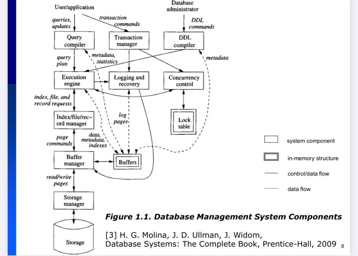
1. DBMS Architecture
2. SQL Index B-Tree
2.1. What index can be cause
-
Increase WHERE qeuery
-
Increase ORDER BY query
-
Increase JOIN query.
-
Auto create index for UNIQUE
CREATE TABLE users ( email VARCHAR(255) UNIQUE );
2.2. Cluster Index
-
What: A clustered index determines the physical order of rows in the table.
-
Store cluster index in a same data page.
-
Primary key: auto create cluster index.
2.3. Secondary Index
- What: A secondary index is a separate structure that points to rows.
| primary_key | |
|---|---|
| a@x.com | 1 |
| b@x.com | 2 |
| c@x.com | 3 |
2.4. How the index is created
CREATE INDEX idx_age ON students(age);
Step 1: Data Collection
Behind the scenes:
- 🔍 Scan toàn bộ table
- 📊 Extract (age, pointer) pairs: [(20,ptr1), (18,ptr2), (22,ptr3)…]
- 🔄 Sort by age: [(17,ptr6), (18,ptr2), (19,ptr4), (20,ptr1)…]
Step 2: Build Tree (Bottom-Up)
📋 Leaf Level: Tạo sorted leaf pages với capacity ~1,300 entries/page 📊 Branch Level: Tạo internal nodes để navigate 📊 Root Level: Single root node pointing to branches
Final result: Balanced tree với height = ⌈log2(records)⌉
Step 3: Point from index to row
Index on name:
Alice → pointer to row 1 Bob → pointer to row 2 Charlie → pointer to row 3
Example:
Pointer Structure: (Page_ID, Slot_Number, Record_Length) Example: ptr1 = (Page_51, Slot_3, 128_bytes)
📄 Data Page 51:
┌─ Slot Directory ─────────────────┐
│ Slot 1 → Offset: 128 │
│ Slot 2 → Offset: 200 │
│ Slot 3 → Offset: 272 ← ptr1 │
│ Slot 4 → Offset: 344 │
├─ Records Data ──────────────────┤
│ @Offset 272: Alice’s record │ ← 128 bytes
└──────────────────────────────────┘
2.5. Cluster Index (Primary Key)
🌳 PRIMARY KEY B-Tree:
[ROOT: id ranges]
/
[BRANCH: id≤1000] [BRANCH: id>1000]
/ | \ / |
📄DATA 📄DATA 📄DATA 📄DATA 📄DATA 📄DATA
Page51 Page52 Page53 Page54 Page55 Page56
📄 Data Page 51 (actual records, sorted by id): [id:1,name:”Alice”,age:20][id:2,name:”Bob”,age:18][id:3,name:”Charlie”,age:22]
= No separate pointer needed!
2.6. Secondary Index:
🌿 Secondary Index (age): 📋 Leaf Pages: [age:17→id:5][age:18→id:2][age:19→id:4][age:20→id:1][age:21→id:3] ↓ ↓ ↓ ↓ ↓ Points to PRIMARY KEY values, not direct page locations
Query execution:
- age=20 → finds id=1 from secondary index
- id=1 → lookup in clustered index for actual data
2.7. Composite Indexes & Leftmost Prefix
CREATE INDEX idx_age_gpa ON students(age, gpa);
🌳 Composite B-Tree: Leaf level sorted hierarchically: [(20,3.2)→id:2][(20,3.5)→id:1][(20,3.5)→id:4][(21,3.2)→id:5][(21,3.5)→id:3] ↑ ↑ ↑ ↑ ↑ age first, then gpa within same age
2.8. Column Order Strategy:
– Query pattern analysis:
– 30% queries: WHERE age = ?
– 40% queries: WHERE age = ? AND gpa >= ?
– 10% queries: WHERE age = ? AND gpa >= ? AND major = ?
– Optimal design: CREATE INDEX idx_age_gpa_major ON students(age, gpa, major); – Covers 80% of query patterns efficiently!
– Wrong design:
CREATE INDEX idx_major_gpa_age ON students(major, gpa, age);
– Only covers 10% efficiently!
2.9. What is right Primary Key
2.9.1. Clustered Index: Must Order in B-Tree
-
Clustered = Data pages physically ordered by index key
-
InnoDB: PRIMARY KEY is always clustered
2.9.2. Could we add primary key for field note/description ?
-
It break to multiple pages.
-
Fewer Index Entries Per Page
Suppose page size is 16KB.
With 8-byte keys: ~1000 entries per page
With 1000-byte keys: ~10 entries per page
So tree becomes:
- taller
- more pages
- more memory usage
- more disk reads
2.9.3. Should we add PRIMARY KEY(country, city, street, zipcode, email)
-
No.
-
In InnoDB, secondary index stores:
(phone_number, country, city, street, zipcode, email)
2.10. Covering Index (query in secondary index is enough)
- If you want to get (secondary_index, primary_key): it is enough, do not read the data page.
2.11. Partial Indexes
– Index only active records CREATE INDEX idx_active_users ON users(last_login) WHERE status = ‘active’;
– Index only recent data
CREATE INDEX idx_recent_orders ON orders(created_date)
WHERE created_date >= ‘2024-01-01’;
2.12. Expression Indexes:
– Index on computed values CREATE INDEX idx_full_name ON users(CONCAT(first_name, ‘ ‘, last_name));
– Case-insensitive search CREATE INDEX idx_email_lower ON users(LOWER(email));
2.13. Why to use composite indexes for multi-column filters
- Without composite index:
Maybe DB uses only: INDEX(customer_id)
Then:
- find all rows for customer 10

- scan them

- filter status='PAID'
- With composite index:
(customer_id, status)
Index is sorted like:
(10, PAID) (10, PENDING) (11, PAID)
Database can jump directly to:
(10, PAID)
Much less scanning.
3. Height of B-Tree:
Suppose:
- page size = 16KB
- each index entry ≈ 12 bytes
Then one index page can store roughly:
-
16000 / 12 ≈ 1333 keys
-
So each node can point to about 1333 child pages.
📈 Tree Height vs Performance:
Records | Tree Height | Max I/O Ops
1,000 | 1 | 1-2
100,000 | 2 | 2-3
10,000,000 | 3 | 3-4
1,000,000,000| 4 | 4-5
Formula: height ≈ ⌈log₁₃₃₃(records)⌉
4. Query optimization using index: No index -> covering index
– Benchmark: 1M records table
Query: SELECT * FROM products WHERE category_id = 5 AND price > 100;
❌ No index (Full table scan):
- I/O operations: 15,000+ (scan all pages)
- Time: 2-5 seconds
- CPU: High (filter every record)
✅ Single index on category_id:
- I/O operations: ~500 (scan matching categories, filter price)
- Time: 100-200ms
- CPU: Medium (filter price for category matches)
✅ Composite index (category_id, price):
- I/O operations: ~50 (direct range scan)
- Time: 10-20ms
- CPU: Low (pre-filtered results)
✅ Covering index (category_id, price, name, description):
- I/O operations: ~25 (index-only scan)
- Time: 5-10ms
- CPU: Minimal
Performance scaling: 500x improvement từ no-index đến covering index!
5. Write Performance Impact:
– Table với multiple indexes:
CREATE TABLE products (
id INT PRIMARY KEY,
name VARCHAR(100),
category_id INT,
price DECIMAL(10,2),
created_date DATE,
INDEX idx_category (category_id),           -- Index #2
INDEX idx_price (price),                    -- Index #3
INDEX idx_date (created_date),              -- Index #4
INDEX idx_composite (category_id, price)    -- Index #5 );
INSERT performance impact:
- No indexes: 1,000 inserts/second
- 5 indexes: ~200 inserts/second (5x slower)
- Storage overhead: ~40% additional space
Trade-off: Faster reads vs slower writes
6. Index Design Rules
✅ DO:
– Analyze query patterns first
– Create indexes for WHERE, ORDER BY, JOIN columns
– Use composite indexes for multi-column filters
– Consider covering indexes for hot queries
– Put most frequently filtered columns first in composite indexes
– Keep PRIMARY KEY narrow and sequential
– Monitor index usage and remove unused indexes
❌ DON’T: – Create indexes on every column “just in case” – Ignore the leftmost prefix rule – Use random UUIDs as PRIMARY KEY – Create redundant indexes – Forget about write performance impact – Create covering indexes for rarely used queries
7. Checklist for Perfomance Optimization
🔍 For each slow query:
- Check if WHERE columns have indexes
- Verify optimal composite index column order
- Consider covering index opportunity
- Analyze EXPLAIN output for full scans
- Monitor index hit ratios
- Look for unused or duplicate indexes
🎯 For each new feature:
- Identify query patterns early
- Design indexes before going to production
- Test with realistic data volumes
- Monitor performance metrics
- Plan for data growth (index maintenance)
8. Core Concepts
- B-Tree = Balanced Search Structure
- O(log n) search performance
- Supports both point and range queries
- Self-balancing for consistent performance
- Index Types Matter
- Clustered (PRIMARY KEY): Data IS the index
- Secondary: Pointers to clustered index
- Composite: Multi-column indexes với leftmost prefix rule
- Covering: All needed columns in index
- Design Principles
- Query patterns drive index design
- Column order matters in composite indexes
- Trade-off between read speed vs write speed
- Monitor usage và remove unused indexes
- When to Use What:
- Point queries: 100-1000x faster với proper index
- Range queries: 10-100x faster
- Covering indexes: 2-10x faster than regular indexes
- Clustered range scans: 10-100x faster than random I/O
🌳 Clustered Index: Always design good PRIMARY KEY
📋 Single Index: Simple WHERE conditions
🔗 Composite Index: Multi-column WHERE, complex queries
📊 Covering Index: Frequent queries với predictable columns
🎯 Partial Index: Filtered datasets, conditional logic
9. Query Optimization
Query Mẫu:
SELECT e.name, d.dept_name FROM employees e JOIN departments d ON e.dept_id = d.id WHERE e.salary > 50000;
Database Có Thể Chọn Nhiều Chiến Lược:
Chiến Lược 1: Nested Loop Join
- Quét toàn bộ bảng employees
- Với mỗi employee có salary > 50000:
- Tìm department tương ứng trong bảng departments
- Trả về kết quả
Cost: Phù hợp khi employees nhỏ, departments có index tốt
Chiến Lược 2: Hash Join
- Tạo hash table từ bảng departments (nhỏ hơn)
- Quét bảng employees, filter salary > 50000
- Với mỗi employee, lookup trong hash table
- Trả về kết quả
Cost: Phù hợp khi có đủ memory, departments vừa phải
Chiến Lược 3: Sort-Merge Join
- Sort bảng employees theo dept_id (có filter salary > 50000)
- Sort bảng departments theo id
- Merge 2 bảng đã sort
- Trả về kết quả
Cost: Phù hợp khi ít memory, data lớn
Execution Plan Components:
📋 Execution Plan Details:
├── 🔍 Access Methods (Table Scan, Index Scan, Index Seek)
├── 🔗 Join Algorithms (Nested Loop, Hash Join, Merge Join)
├── 📊 Sort Operations (ORDER BY, GROUP BY)
├── 🎯 Filter Operations (WHERE conditions)
├── 📈 Cost Estimates (CPU, I/O, Memory)
└── ⏱️ Execution Order (Step-by-step sequence)
10. Explain query
Cách Xem Execution Plan: – Basic explain EXPLAIN SELECT e.name, d.dept_name FROM employees e JOIN departments d ON e.dept_id = d.id WHERE e.salary > 50000;
– Detailed JSON format EXPLAIN FORMAT=JSON SELECT …;
+—-+————-+——-+——+—————+——+———+——+——+————-+ | id | select_type | table | type | possible_keys | key | key_len | ref | rows | Extra | +—-+————-+——-+——+—————+——+———+——+——+————-+ | 1 | SIMPLE | e | ALL | dept_id | NULL | NULL | NULL | 1000 | Using where | | 1 | SIMPLE | d | ref | PRIMARY | PRIMARY | 4 | e.dept_id | 1 | NULL | +—-+————-+——-+——+—————+——+———+——+——+————-+
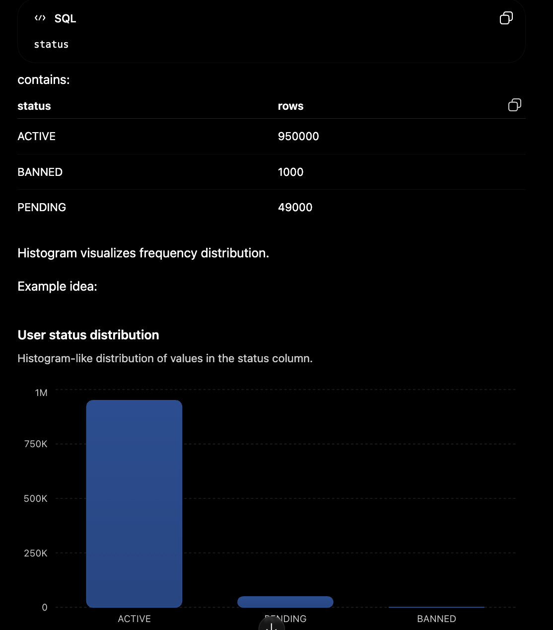
11. Histogram MySQL
Show distribution of SQL value before making decisions
– Force update statistics ANALYZE TABLE employees;
– Với sampling cho table lớn: ANALYZE TABLE employees UPDATE HISTOGRAM ON salary, dept_id WITH 100 BUCKETS;
– Xem chi tiết histogram:
SELECT
schema_name,
table_name,
column_name,
JSON_EXTRACT(histogram, ‘$.buckets’) as histogram_buckets
FROM information_schema.column_statistics
WHERE table_name = ‘employees’;
12. Query Processing Plan
Bước 1: Parse (Phân Tích Cú Pháp)
-
Mục đích: Kiểm tra tính đúng đắn về mặt cú pháp SQL
-
Ví dụ:
– ✅ ĐÚNG SELECT * FROM employee WHERE emp_id = 100;
– ❌ SAI SELCT * FROM employee WHERE emp_id = 100; – Lỗi: ORA-00923
Bước 2: Validate (Kiểm Tra Ngữ Nghĩa)
- Mục đích: Xác minh sự tồn tại của table, column, permissions
Kiểm tra:
- Bảng employee có tồn tại không
- Cột emp_id có trong bảng không?
- User có quyền truy cập không?
Lỗi phổ biến: ORA-00942: table or view does not exist
Bước 3: Shared Pool Check
-
Mục đích: Tìm kiếm execution plan đã có sẵn
-
Kết quả:
FOUND → Soft Parse (nhanh) NOT FOUND → Hard Parse (chậm)
Bước 4: Hard Parse (Nếu Cần)
-
Mục đích: Tạo execution plan tối ưu
-
Quy trình:
- Phân tích các chiến lược thực thi
- Chọn plan tối ưu nhất
- Tính toán cost và statistics
Bước 5: Store Plan
-
Mục đích: Lưu execution plan vào Shared Pool
-
Lợi ích: Tái sử dụng cho các lần thực thi sau
Bước 6: Execute
-
Mục đích: Thực thi câu lệnh và trả về kết quả
-
Hoạt động: Truy xuất dữ liệu từ storage theo plan
Example:
– ❌ Những câu này được coi là KHÁC NHAU:
SELECT * FROM employee WHERE emp_id = 100 Select * from employee where emp_id = 100 – Khác case SELECT * FROM EMPLOYEE WHERE EMP_ID = 100 – Khác case select * from employee where emp_id=100 – Thiếu space
13. Hard Parse and Soft Parse difference
13.1. Hard Parse
A hard parse happens when the database must fully process a SQL query from scratch.
Steps include:
- syntax check
- semantic check (tables/columns exist)
- permissions check
- generate execution plan
- optimize query
- store plan in cache
13.2. Soft Parse
A soft parse happens when the database reuses an existing execution plan from cache.
Instead of rebuilding everything:
- DB finds cached SQL plan
- validates it
- executes directly
14. InnoDB Storage
14.1. File of table
📁 /var/lib/mysql/ (Linux) hoặc C:\ProgramData\MySQL\ (Windows)
├── 📁 mysql/ ← System database
├── 📁 performance_schema/ ← Performance monitoring
├── 📁 hanzi/ ← User database
│ ├── admins.ibd (112 KB) ← Table files
│ ├── category.ibd (144 KB)
│ ├── e_questions.ibd (21 MB) ← Hot table
│ ├── e_answers.ibd (10 MB) ← Hot table
│ └── db.opt ← Database config
├── 📄 ib_logfile0 ← Transaction log #1
├── 📄 ib_logfile1 ← Transaction log #2
├── 📄 ibdata1 ← System tablespace
└── 📄 binlog.000001 ← Binary logs
- Term .ibd: InnoDB data file
14.2. Store by page
📄 Mỗi tệp .ibd được chia thành các trang (16KB mỗi trang):
Trang 0: Tiêu đề tệp + Metadata
Trang 1: Gốc Index chính
Trang 2: Gốc các Index phụ
Trang 3-N: Trang dữ liệu
14.3. Execute plan
Note: need to load data from data page -> Memory to query.
SELECT * FROM user WHERE id = 100;
Bước 1: 🧠 Phân tích Truy vấn (Bộ nhớ)
✅ Phân tích cú pháp SQL
✅ Kiểm tra sự tồn tại của bảng/cột
✅ Chọn kế hoạch thực thi
Bước 2: 💿→🧠 Tải Trang từ Ổ đĩa MySQL KHÔNG đọc trực tiếp từ ổ đĩa!
- Tải trang từ ổ đĩa → Vùng đệm (RAM)
- Xử lý dữ liệu trong bộ nhớ
- Trả về kết quả
Bước 3: 🧠 Xử lý Dữ liệu (Bộ nhớ) Các thao tác CPU trong RAM:
- Phân tích nội dung trang
- Lọc bản ghi theo điều kiện WHERE
- Trích xuất các cột cần thiết
Thời gian Hiệu suất
💿 I/O ổ đĩa: ~10ms (tải trang) 🧠 Xử lý RAM: ~0.001ms (xử lý dữ liệu)
= I/O ổ đĩa chậm hơn 10,000 lần!
15. Parition Data in SQL
📁 Thư mục Database:
├── orders#P#p2021.ibd ← Dữ liệu 2021
├── orders#P#p2022.ibd ← Dữ liệu 2022
├── orders#P#p2024.ibd ← Dữ liệu 2024
└── orders#P#p2025.ibd ← Dữ liệu 2025
16. Strategy for multiple file data
🔥 Dữ liệu NÓNG (Truy cập thường xuyên):
- Dữ liệu kỳ học hiện tại (e_questions, e_answers)
- Phiên người dùng, xác thực
- Giao dịch đang hoạt động
🌤️ Dữ liệu ẤM (Truy cập vừa phải):
- Dữ liệu kỳ học gần đây
- Hồ sơ người dùng
- Dữ liệu cấu hình
❄️ Dữ liệu LẠNH (Truy cập hiếm):
- Dữ liệu lịch sử (>1 năm)
- Nhật ký kiểm toán
- Tệp sao lưu
📊 Kiến trúc Phân tầng: Tầng 1 - NVMe SSD (D:): Dữ liệu nóng ├── Chi phí: $100/TB ├── Tốc độ: 3,500 MB/s └── Sử dụng: Các thao tác thời gian thực
Tầng 2 - SATA SSD (E:): Dữ liệu ấm
├── Chi phí: $60/TB
├── Tốc độ: 500 MB/s
└── Sử dụng: Báo cáo, thao tác quản trị
Tầng 3 - HDD (F:): Dữ liệu lạnh
├── Chi phí: $20/TB
├── Tốc độ: 150 MB/s
└── Sử dụng: Lưu trữ, tuân thủ
16.1. Implement hot, warm, cold data
– Tạo các tablespace phân tầng CREATE TABLESPACE hot_tier ADD DATAFILE ‘D:\MySQL\Hot\hot.ibd’; CREATE TABLESPACE warm_tier ADD DATAFILE ‘E:\MySQL\Warm\warm.ibd’; CREATE TABLESPACE cold_tier ADD DATAFILE ‘F:\MySQL\Cold\cold.ibd’;
– Phân phối bảng theo mẫu truy cập
ALTER TABLE e_questions TABLESPACE hot_tier; – Tần suất cao
ALTER TABLE e_exams TABLESPACE warm_tier; – Tần suất vừa
ALTER TABLE audit_logs TABLESPACE cold_tier; – Tần suất thấp
– Partition large tables với tiered storage CREATE TABLE e_questions_new ( question_id INT, exam_id INT, created_date DATE ) PARTITION BY RANGE (YEAR(created_date)) ( PARTITION p2024 VALUES LESS THAN (2025) TABLESPACE hot_tier, PARTITION p2025 VALUES LESS THAN (2026) TABLESPACE hot_tier, PARTITION p2022 VALUES LESS THAN (2023) TABLESPACE cold_tier, PARTITION p2021 VALUES LESS THAN (2022) TABLESPACE cold_tier );
17. Prepare statements
Phase 1: PREPARE (Chỉ 1 lần)
- Parse → Kiểm tra cú pháp
- alidate → Kiểm tra table/column
- Optimize → Tạo execution plan
- Store → Lưu plan vào memory
Phase 2: EXECUTE (Nhiều lần)
- Bind values → Gán giá trị cho placeholder
- Execute → Chạy với plan có sẵn