



Advanced Global Distributed System - Consensus Algorithm, Concepts
Here is learning concepts for distributed system through implementation.
1. The Messenger
1.1. Design a system where multiple services communicate reliably without shared memory. What primitives would you use and why?
-
Shared memory: in same machine
-
Message passing: different machines.
Answer: Message queues (Kafka, SQS) for async decoupling; gRPC/HTTP for synchronous RPCs. Each message must be self-contained. Discuss at-least-once vs at-most-once delivery, idempotency keys to handle retries, and correlation IDs for request tracing across services.
1.2. How does a service know which message it received is a response to a specific request it sent earlier?
Answer: Correlation/request IDs: the sender attaches a unique ID to each outgoing request. The receiver echoes this ID in its response. The sender maps incoming response IDs to pending callbacks. This is how HTTP/2 stream IDs, Kafka consumer group offsets, and Maelstrom msg_ids all work.
- How to know the client
- Using request id.
- How to know the offset of multiple packets
-
Sequence number: the byte that send in the payload.
-
Acknowledge number: the byte is expected next.
1.3. A service sends a request and never gets a response. How do you decide whether to retry?
-
Use timeouts with exponential backoff and jitter. Retry only idempotent operations (GET, PUT with full replacement) or operations with idempotency keys.
-
Use circuit breakers to stop retrying against a consistently failing downstream. Distinguish between 503 (retry) and 400/404 (do not retry).
1.4. What is the difference between a message broker and a service mesh? When would you choose each?
-
A message broker (Kafka, RabbitMQ) provides async, durable message delivery with decoupled producers and consumers.
-
A service mesh (Istio, Linkerd) handles synchronous service-to-service traffic with features like mTLS, retries, circuit breaking, and observability.
-
Use a broker when you need temporal decoupling or fan-out; use a mesh for sync RPC with cross-cutting network concerns.
1.5. How would you debug a system where messages are being processed more than once?
-
Check for duplicate delivery: is the queue at-least-once? Is the consumer crashing after processing but before acknowledging?
-
Add idempotency: track processed message IDs in a store and skip duplicates.
-
Use exactly-once semantics in Kafka (requires transactions + idempotent producers) for critical flows.
-
Log message IDs at each processing step to trace duplicates.
1.6. Serialisation Message: JSON vs Protobuf vs MessagePack
| Dimension | JSON | Protobuf | MessagePack |
|---|---|---|---|
| Human readable | ✅ Yes | ❌ No (binary) | ❌ No (binary) |
| Payload size | Large (field names repeated) | Small (field tags, no names) | Medium (compact binary JSON) |
| Parse speed | Slow | Fast | Fast |
| Schema required | No | Yes (.proto file) |
No |
| Schema evolution | Flexible but fragile | Excellent (field numbers) | Good if using maps; fragile if using arrays |
| Debugging ease | Easy (curl, browser) | Hard (need .proto) |
Hard (binary) |
| Best for | REST APIs, prototyping | gRPC, high-throughput microservices | Cache serialization, Redis, IPC |
Verdict: Start with JSON for correctness, migrate to Protobuf when payload size or parse latency becomes a bottleneck.
Example:
JSON:
{
  "id": 123,
  "name": "Alice",
  "active": true
}
Message Pack:
map(3)
string("id")
int(123)
string("name")
string("Alice")
string("active")
true
1.7. Transport: TCP or UDP
| Dimension | TCP | UDP |
|---|---|---|
| Delivery guarantee | Exactly once (at the OS level) | Best effort — packets may be lost |
| Ordering | In-order delivery guaranteed | Out-of-order delivery possible |
| Latency | Higher (3-way handshake, retransmissions, ACKs) | Lower (fire-and-forget) |
| Head-of-line blocking | Yes — one lost packet blocks subsequent packets until it is retransmitted | No — each datagram is independent |
| Connection setup | Connection-oriented (3-way handshake required) | Connectionless (first packet is sent immediately) |
| Flow & congestion control | Built-in (sliding window, congestion control) | None (application must implement if needed) |
| Reliability | Reliable (ACKs + retransmissions) | Unreliable (no ACKs or retransmissions) |
| Packet boundaries | Byte stream (no message boundaries) | Datagram-oriented (message boundaries preserved) |
| Header size | 20–60 bytes | 8 bytes |
| Typical use cases | HTTP/HTTPS, databases, file transfer, email, SSH | DNS, VoIP, video streaming, online gaming, QUIC |
Verdict: TCP for reliability by default. UDP only when you implement your own reliability layer (like QUIC) or can tolerate loss (metrics, video).
1.8. Why Grpc sync call needed timeout:
-
Sends a message to another node
-
Blocks until a response is received (matched by in_reply_to)
-
Returns the response body
-
Times out after a configurable duration (default: 1 second)
1.7. Why server know what client request id
-
Add request id in the header.
-
Server response: what the client it reply to.
1.8. What is asynchronous RPC callback ?
-
Sends a message to a target node
-
Registers a callback function keyed by the outgoing msg_id
-
Returns immediately (non-blocking)
-
When a reply arrives (with matching in_reply_to), invokes the callback with the reply body
1.9. What is callback reaper to store message, when recipient crashes or the network drops ?
- DLQ for failure process consumer.
1.10. How server handle callback reaper ?
-
Records the timestamp when each callback is registered
-
Periodically scans for callbacks older than a threshold (default: 2 seconds)
-
Removes expired callbacks and invokes them with a timeout error
-
Reports how many callbacks were reaped
1.11. Using add jitter for thunderherd retry
- Add jitter for pods do not retry at the same time.
1.12. JSON Encode from and to Byte
-
Merge from byte -> data structure: int, string, map.
-
Convert it to JSON again.
1.13. Log for message tracing
- Add request, response and message_type.
1.14. Deduplication in network layer using LRU Cache
-
Dedup by using (src, msg_id).
-
But use LRU for dedup it -> but around message IDs (capacity: 1000)
1.15. Chaos Testing - Drop network packet loss
- When chaos mode is enabled, the node randomly drops a configurable percentage of outgoing messages (does not send them to stdout)
1.16. Benchmark Node Throughput and Latency
- Benchmark latency and throughput per node.
1.17. Story
1.17.1. gRPC communicate
Every RPC call you make in production, from your app server to the database and back, follows the same request/response pattern you are implementing here. Slack processes over 1 billion messages per day through exactly this kind of node-to-node messaging layer. Getting the message format and routing right is the foundation everything else sits on.
Used in: Slack, Discord, gRPC
1.17.2. Correlation IDs
Correlation IDs are how distributed tracing works. When a request to netflix.com triggers 50 downstream service calls, each call carries the same correlation ID. Without it, tracing a single user request across a distributed system is effectively impossible. You are building that primitive now.
Used in: Netflix, Jaeger, Zipkin
1.17.3. Retry with exponential backoff and jitter
Retry logic with exponential backoff and jitter is in every production service. When AWS has a partial outage, the difference between a retry storm that worsens the outage and a graceful degradation is jittered backoff. Stripe’s payment retries, AWS SDK retries, and gRPC’s retry policy all implement what you are building here.
Used in: Stripe, AWS SDK, gRPC
1.17.4. Broadcast CDC
Broadcast is how database change data capture (CDC) works. When Debezium detects a row change in Postgres, it broadcasts that change event to every downstream consumer. The broadcast semantics you implement here are the same ones that power real-time analytics at Uber and DoorDash.
Used in: Debezium, Uber, DoorDash
1.17.5. Network partition is not rare
Network partitions are not rare. AWS us-east-1 has had at least 12 documented network partition events in the past five years. Every major distributed system must handle the case where some nodes can communicate with each other but not others. What you build here determines whether your system degrades gracefully or corrupts data silently.
Used in: AWS, Google Cloud, Azure
2. The Identifier
2.1. Story
2.1.1. Unique tracing for activity id
Instagram generates over 100 million posts per day. Each post, comment, and like needs a globally unique ID generated without any coordination between servers. Before they built their Snowflake-inspired generator, insert latency was dominated by the ID generation step. You are solving the same problem.
Used in: Instagram, Twitter, Discord
2.1.2. UUID v4 and Snowflake timestamp (UUID v7)
UUID v4 is random — it does not sort by time. When you index 10 billion UUID v4 rows in PostgreSQL, every insert causes a page split somewhere in the B-Tree because the new value lands at a random position. This destroys write performance at scale. UUID v7, ULID, and Snowflake all exist specifically to solve this problem.
Used in: PostgreSQL, CockroachDB, Cassandra
| timestamp | machine | sequence | +————+———–+———–+
2.1.3. Random sequence number from worker start
Discord generates 100 million unique IDs per day for messages alone. Their Snowflake implementation uses a 10-bit worker ID that encodes datacenter and process. When a worker process restarts, it must avoid reusing a sequence number — the subtle monotonicity guarantee you are implementing now prevents phantom duplicates in their message history.
Used in: Discord, Snowflake, Twitter
2.1.4. Vector Clocks (Order of event happened), not Clock Drift (in case GMT + 0)
Vector clocks are the foundation of Amazon DynamoDB’s conflict resolution and Apache Cassandra’s last-write-wins logic. When two clients write to the same key during a network partition, the system needs to know which write is causally later. Without a proper causal ordering mechanism, you get silent data corruption.
Used in: Amazon DynamoDB, Apache Cassandra
2.1.5. NTP clock skew problem
The NTP clock skew problem is not theoretical. In 2012, a leap second event caused Linux kernels to spin at 100% CPU because the clock jumped backward, breaking monotonicity assumptions in the kernel’s scheduler. Your ID generator must handle backward clock jumps without producing duplicate IDs.
Used in: Linux kernel, Cloudflare, Reddit
2.2. Self-node generated ID, do not need coordination or other nodes
- Generated IDs must be globally unique - use timestamp + node_id + sequence to guarantee no collisions even under partition
2.3. Using custom epoch, not Unix epoch for Snowflake ID -> timestamp (41 bit)
-
Due to since (1970-01-01) -> today: 56 years.
-
But in 2^41 bit -> can store 69 years, we have used 56 years -> 13 years only.
=> custom epoch to go again.
2.4. Sequence number (12 bit) can from 1 -> 4096
- After full the sequence number -> update it.
2.5. Machine number bit -> 10 bit.
- You can 1024 unique machines generating IDs
2.6. Lamport clocks
P2 = max(2,4) + 1 = 5
P1 P2 P3
1 2 3 4(send) ——>
           5(receive)
           6(send) ----->

                           7(receive)
2.6. Lamport clocks limit: if A happens-before B, then L(A) < L(B). But the converse is not true
- So do not know relationship between event: A,B,C based on L(A), L(B), L(C)
2.7. Vector clocks
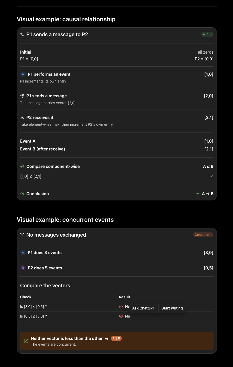
2.8. Riak DB - Detect write conflicts - Vector Clocks
- In databases like Riak, vector clocks detect write conflicts. When two clients write to the same key concurrently (neither saw the other’s write), the database stores both values as siblings instead of silently losing one.
{"type": "vc_read_ok", "values": [
    {"value": "a", "vc": {"n1": 1}},
    {"value": "b", "vc": {"n2": 1}}
], "siblings": 2}
2.9. CockroachDB and Spanner - Hybrid Logical Clocks (HLC)
-
Vector clocks: ordering: A < B, A B. - Physical clock: what time it happened.
A Hybrid Logical Clock (HLC) timestamp consists of two values:
HLC = (l, c)

l = logical/physical timestamp (milliseconds)
c = logical counter
l: The maximum physical time observed by the node.c: A logical counter used to preserve causality when physical time alone is insufficient.
Algorithm 1: Local Event
Whenever a local event occurs (e.g., writing to a database), update the HLC as follows:
pt = current physical time

if pt > l
    l = pt
    c = 0
else
    c = c + 1

return (l, c)
Example 1: Physical Clock Advances
Current HLC:
(1000, 0)
Current physical time:
1001
Since:
1001 > 1000
Update the HLC:
(1001, 0)
Example 2: Physical Clock Does Not Advance
Current HLC:
(1001, 0)
Current physical time:
1001
Since:
pt == l
Increment the logical counter:
(1001, 1)
Another local event within the same millisecond:
(1001, 2)
Algorithm 2: Sending a Message
When sending a message, attach the current HLC timestamp.
Message
{
    payload,
    timestamp = (l, c)
}
The sender’s HLC is not modified when sending.
Algorithm 3: Receiving a Message
Suppose Node A sends the following timestamp:
(1005, 3)
Node B currently has:
Physical Clock = 1002

HLC = (1002, 1)
When Node B receives the message, it first computes:
l' = max(
    local physical time,
    local HLC.l,
    received HLC.l
)
For this example:
max(
    1002,
    1002,
    1005
)
=
1005
After computing l', there are three possible cases.
Case 1: Received Timestamp Is the Largest
Condition:
received.l == l'
Update:
l = received.l
c = received.c + 1
Example:
Received HLC : (1005, 3)

Result:

(1005, 4)
This preserves the causal relationship:
A sends      (1005, 3)
      │
      ▼
B receives   (1005, 4)
Case 2: Local HLC Is the Largest
Condition:
local.l == l'
Update:
l = local.l
c = local.c + 1
Example:
Local HLC    : (1005, 7)
Received HLC : (1002, 5)

Result:

(1005, 8)
Case 3: Physical Clock Is the Largest
Condition:
physical time == l'
Update:
l = physical time
c = 0
Example:
Physical Clock : 1008
Local HLC      : (1006, 2)
Received HLC   : (1005, 7)

Result:

(1008, 0)
Since the physical clock has naturally advanced, the logical counter is reset.
Complete Receive Algorithm
receive(message)

pt = current physical time

l' = max(
    pt,
    local.l,
    message.l
)

if l' == pt
    l = pt
    c = 0

else if l' == local.l
    l = local.l
    c = local.c + 1

else
    l = message.l
    c = message.c + 1

return (l, c)
Summary
| Event | Update Rule |
|---|---|
| Local event | Advance physical time if possible; otherwise increment logical counter. |
| Send message | Attach current HLC timestamp. |
| Receive message | Take the maximum of local physical time, local HLC, and received HLC, then update the logical counter according to the winning timestamp. |
The HLC algorithm guarantees that if event A causally happens before event B (A → B), then:
HLC(A) < HLC(B)
2.10. Why we have HLC clock
-
Store (physical_ms, logical_count)
-
Vector clocks are actually more powerful than HLC. HLC was not invented because vector clocks are wrong—it was invented because vector clocks become impractical in large distributed systems.
-
Trade-offs: not correctness but sclability
-
HLC does not eliminate clock drift. It only ensures that causal ordering is preserved despite clock drift.
2.11. Design a globally unique ID generator that produces sortable IDs without a central coordinator.
- Snowflake-style: 41-bit millisecond timestamp + 10-bit machine ID (datacenter + worker) + 12-bit sequence. Gives 4096 IDs/ms/machine, IDs sort by time, no coordination. Alternatives: ULIDs (128-bit, base32 encoded, monotonic within millisecond), UUID v7 (timestamp-first UUID). Discuss clock drift and the monotonicity problem when NTP steps the clock backward.
2.12. Why is using auto-increment IDs in a sharded database a problem? How do you solve it?
- Auto-increment requires a central sequence generator, which is a single point of failure and a scaling bottleneck. Solutions: distributed ID generators (Snowflake), UUIDs (random, no coordination but poor index locality), shard-aware IDs that encode shard ID. Instagram used Postgres sequences per shard with a large step size to avoid coordination.
2.13. What happens to your ID generator when the system clock moves backward due to an NTP sync ? - Can not
- If time moves backward, you might generate a duplicate ID (same timestamp + same sequence). Snowflake’s solution: detect backward clock movement (currentTime < lastTimestamp), then wait until the clock catches up. Some implementations add a machine-restart counter to the ID. Hybrid Logical Clocks (HLCs) use max(wallClock, lastSeenHLC) to stay monotonic even across NTP adjustments.
2.14. A UUID has 122 bits of randomness. What is the probability of a collision if you generate 1 billion UUIDs?
- The birthday problem: with n IDs drawn from a space of size N = 2^122, the collision probability is approximately 1 - e^(-n^2 / 2N). With n = 10^9, this is about 10^18 / (2 * 2^122) ≈ 10^-19. Effectively zero. In practice, UUID collisions are so rare that the RNG quality matters more than the math.
2.15. Why do random UUIDs perform poorly as database primary keys compared to sequential IDs?
- B-tree indexes store keys in sorted order. Random UUIDs insert into random positions, causing frequent page splits and fragmentation. Sequential IDs always append to the right of the B-tree, maximizing page fill and minimizing splits. Impact: 3-5x write throughput difference on high-insert workloads. Solution: use time-sortable IDs (Snowflake, ULID, UUID v7) which have the uniqueness of UUIDs with the sequential insert properties of auto-increment.
3. The Gossiper
3.1. Story
3.1.1. Cassandra - Gossip for all
Apache Cassandra uses gossip to propagate cluster membership, token ranges, and schema changes to every node. When you add a new Cassandra node to a 100-node cluster, the gossip protocol ensures every other node knows about it within seconds — without any central coordinator. This is the broadcast mechanism you are implementing.
Used in: Apache Cassandra, Consul
3.1.2. HashiCorp - Tree Topology Gossip
Serf, HashiCorp’s cluster membership library, uses a tree topology for initial broadcast to limit the number of messages before switching to gossip for reliability. The two-phase approach you are building here is exactly what real cluster membership protocols use to balance speed with fault tolerance.
Used in: HashiCorp Serf, Consul, Nomad
- With Cassanra gossip:
1 node - all nodes
...

Eventually everyone learns.
- With tree gossip:
       A
      /|\
     / | \
    B  C  D
   / \ | / \
  E  F G H I

Later...

C → E
D → E
F → E
3.1.3. Redis Cluster - Random Gossip
Redis Cluster uses gossip to propagate cluster state across up to 1000 nodes. Each node sends a PING to a random selection of other nodes every second, embedding state about nodes it has not heard from recently. The random gossip strategy you are implementing is directly applicable to Redis Cluster’s failure detection.
Used in: Redis Cluster, etcd
Round 1
Every second, node A randomly selects a few peers.
For example:
A
├──► C
└──► H
The PING message is not just a heartbeat:
PING
It also carries gossip information about other nodes.
Example:
PING

Gossip:
F = FAIL
E = OK
J = OK
After receiving the PING:
C:
F = FAIL

H:
F = FAIL
Round 2
Now C and H also gossip to randomly selected peers.
For example:
C
├──► D
└──► G

H
├──► B
└──► I
Now these nodes have learned that F has failed:
B knows:
F = FAIL

D knows:
F = FAIL

G knows:
F = FAIL

I knows:
F = FAIL
Round 3
Those nodes continue gossiping to new random peers.
D ──► J

B ──► E

I ──► A

...
Eventually, the information reaches every node:
A  B  C  D  E  F  G  H  I  J

All know:

F = FAIL
Notice that no node ever contacts every other node directly. Instead, the information spreads from node to node like an epidemic, eventually reaching the entire cluster through random peer selection.
3.1.4. CockroachDB - Batch Gossip
CockroachDB batches gossip updates to avoid overwhelming the network when many nodes join or leave simultaneously. Your batching implementation mirrors the same technique CockroachDB uses to keep gossip overhead below 1% of total network bandwidth even in 500-node clusters.
Used in: CockroachDB, TiKV
Batching
Instead of sending immediately, node A waits for a short batching window.
For example:
10 ms
During those 10 ms:
Node B joined

Node C left

Node D updated

Node E changed lease

Node F became healthy
Rather than sending five separate gossip messages:
PING

Update:
B joined
PING

Update:
C left
PING

Update:
D updated
…
A sends one batched message:
PING

Batch:

- B joined
- C left
- D updated
- E lease changed
- F healthy
3.1.5. Amazon DynamoDB - Slow Detect Failure Nodes
The 2013 Amazon DynamoDB “heat” incident happened because node failure detection was too slow during a network partition. Nodes were considered alive longer than they were, causing requests to pile up at dead nodes. The partition-healing gossip you are building now is the mechanism that makes failure detection both fast and accurate.
Used in: Amazon DynamoDB, Riak
3.2. Hybrid Gossip (Tree + Random Catch-up)
Implement a hybrid broadcast:
-
On broadcast, forward via tree neighbors immediately
-
Periodically gossip all known messages to random peers (catch-up)
-
Track delivery path for each message (tree vs gossip)
3.3. Isolated group - Network Partition
Network partitions split the cluster into isolated groups. After the partition heals, gossip must merge the diverged states. Your task is to simulate this.
Implement:
-
partition - Block messages to specified nodes
-
heal - Unblock all nodes
-
partition_status - Report current partition state
3.4. CRDT (Conflict-free Replicated Data Type) - Grow-only Set (G-Set)
A Grow-only Set (G-Set) is the simplest CRDT. Elements can be added but never removed. Merge is set union, which is commutative, associative, and idempotent - guaranteeing eventual consistency via gossip.
3.5. Last-Write win Cassandra (still have Clock Drift)
- Cons: still have clock drift.
3.6. LSM Tree have read performance trade-offs
L0
 ├── SSTable A
 ├── SSTable B
 ├── SSTable C

L1
 ├── SSTable D
 ├── SSTable E

L2
 ├── SSTable F
SSTable is already sorted
+—————-+ | Index Block | +—————-+ | Block 1 | Keys: 1–1000 +—————-+ | Block 2 | Keys: 1001–2000 +—————-+ | Block 3 | Keys: 2001–3000 +—————-+
3.7. LSM Tree Architecture
                   Write Path
                 PUT(key, value)
                        │
                        ▼
                +----------------+
                |   WAL (Disk)   |  ← Durability
                +----------------+
                        │
                        ▼
                +----------------+
                |   MemTable     |  ← In-memory sorted tree
                +----------------+
                        │
                Memory Full?
                        │
                  Yes   ▼
                +----------------+
                | Immutable MT   |
                +----------------+
                        │
                        ▼
               Flush Sequentially
                        │
                        ▼
         +-----------------------------+
         | SSTable (Level 0)           |
         +-----------------------------+
                        │
                  Background
                  Compaction
                        │
                        ▼
         +-----------------------------+
         | Level 1 SSTables            |
         +-----------------------------+
                        │
                        ▼
         +-----------------------------+
         | Level 2 SSTables            |
         +-----------------------------+
                        │
                        ▼
                    ...
3.8. MemTable is already sorted - skip list
- Write in multiple layer -> search faster.
Level 4

3 ----------------------> 50

Level 3

3 -----------> 25 ------> 50

Level 2

3 ---> 15 ---> 25 ---> 40 ---> 50

Level 1

3 -> 8 -> 15 -> 20 -> 25 -> 40 -> 50

Level 0

3 -> 5 -> 8 -> 10 -> 15 -> 18 -> 20 -> 25 -> 30 -> 40 -> 50
3.9. How skip list write data
-
Find index from higher layer.
-
Update data in above layer (double linked list)
Level 2

3 -----------> 12 -----------> 20

Level 1

3 -------> 10 -----> 12 -----> 20

Level 0

3 -> 7 -> 10 -> 12 -> 15 -> 20
3.10. How does Cassandra propagate cluster membership changes? What protocol does it use and what are its guarantees?
Cassandra uses a gossip protocol where each node gossips with three random peers per second. It exchanges Gossip Digest (node + version) in three phases: SYN (send digest), ACK (send missing info), ACK2 (confirm receipt). Convergence time is O(log N) rounds. It provides eventual consistency for cluster state, not strong consistency.
3.11. Design a failure detection system for a cluster of 1000 nodes that detects failures within 10 seconds without false positives.
Use SWIM-style gossip-based failure detection: periodic ping with indirect probing (if direct ping fails, ask k peers to probe). Tunable: ping interval, ping timeout, k for indirect probing. 10-second detection with low false positives requires ping interval around 1-2s. Phi accrual failure detector (used by Akka/Cassandra) maintains a sliding window of heartbeat intervals and computes a suspicion level rather than a binary up/down.
3.12. Compare gossip protocols to centralized cluster management systems (like ZooKeeper). When would you choose each?
Gossip: decentralized, no single point of failure, O(log N) convergence, eventual consistency, scales to thousands of nodes. Used when you can tolerate eventual consistency for cluster state.
ZooKeeper: strongly consistent, linearizable reads, immediate failover detection, but requires a quorum of ZK nodes, has lower write throughput. Use ZooKeeper for configuration, leader election, and distributed locks where strong consistency is required. Use gossip for membership and health state where eventual consistency is acceptable.
3.13. A gossip message takes 3 rounds to reach all nodes in a 1000-node cluster. What is the approximate fanout you are using?
With fanout f and k rounds, the number of informed nodes grows as f^k. For 3 rounds to reach 1000 nodes: f^3 ≈ 1000, so f ≈ 10. In practice you need to account for the proportion already informed, so the actual fanout needed is a bit higher. Typical gossip systems use fanout of 3-5 with more rounds.
3.14. How would you implement gossip-based broadcast that guarantees delivery even if 20% of nodes fail mid-broadcast?
Use push-pull gossip with redundancy: each node gossips to more than 1 peer per round (fanout > 1). With f = 3 and 20% failure rate, the probability of any single path being blocked is 0.2.
After k rounds, the probability of not receiving a message via at least one path decreases exponentially.
Combine with anti-entropy: nodes periodically ask random peers for messages they may have missed (pull). Add message IDs for deduplication. Bloom filters on the receiver side to quickly check “have I seen this ID?”
4. The TimeKeeper
4.1. Story
4.1.1. Spanner - use GPS and atomic clocks for true time
Google Spanner uses GPS receivers and atomic clocks in every data center to bound clock uncertainty to within 7 milliseconds. Before committing a transaction, Spanner waits out this uncertainty window to guarantee that no other transaction globally can have a later timestamp and still be considered concurrent. The physical clock handling you are building here is the foundation of that technique.
Used in: Google Spanner, CockroachDB, YugabyteDB
4.1.2. Clock Drifts - Linux kernels downtime - Cause loop interval to fix the timestamp problem that cause crash server
In 2012, a leap second caused Linux kernels to spin in a busy loop, taking down servers at Reddit, Gawker, LinkedIn, and Qantas simultaneously. The root cause was a clock backward jump that the kernel’s hrtimer did not tolerate. The backward jump detection you are implementing is the kind of defensive code that prevents a routine calendar event from becoming an outage.
Used in: Linux kernel, distributed systems globally
4.1.3. Why Google Spanner introduce TrueTime API
Google’s TrueTime API reports time as an interval [earliest, latest] rather than a single value. Every Spanner server calls TrueTime before acquiring a lock and waits until now.earliest is past the lock’s expiry to guarantee the lease has truly expired globally. The mock TrueTime API you are building captures this uncertainty model precisely.
Used in: Google Spanner, Google Colossus
Why google introduce it ?
earliest = local_clock - ε
latest   = local_clock + ε
The difficult part is how Google knows ε: Using GPS + logical_clock
           GPS Satellites
                 │
          Atomic Clocks
                 │
        Time Master Servers
                 │
        Datacenter Servers
                 │
        Application Servers
4.1.4. How does Spanner calculate ε (epsilon)?
          GPS Satellites
                 │
          Atomic Clocks
                 │
        Time Master Servers
                 │
        ---------------------
        |        |          |
     Server A  Server B  Server C
        │        │          │
     TrueTime  TrueTime  TrueTime
Each server periodically synchronizes with Google’s time masters.
TrueTime continuously estimates:
ε =
    clock drift
  + network delay uncertainty
  + synchronization error
  + hardware oscillator error
  + measurement error
4.1.5. Is [earliest, latest] per transaction?
No. It is per call to TT.now(), not per transaction.
10:00:00.010

TT.now()

↓

[110,113]
4.1.6. If intervals overlap, how does Spanner detect which event happened first?
Case 1: [curr_1, latest_1] < [curr_2, latest2] in case latest_1 < curr_2 => it make sense.
Case 2::
TA: 100---------105
 TB:     103---------108
Then how does Spanner decide?
-
Spanner uses transaction coordination (based on Paxos).
-
Force transaction commit after: curr_2 > latest_1
Client 1

↓

Transaction A

↓

Paxos leader

↓

Assign commit timestamp = 105

↓

Commit wait

↓

TT.now() = [106,111]

↓

Return success
Client 2

↓

Transaction B

↓

Starts after Client 1 received success

↓

TT.now() = [107,112]

↓

Timestamp must be >105
4.1.7. Google Spanner - The “wait-out-uncertainty” technique
The “wait-out-uncertainty” technique in Spanner ensures that a write committed at timestamp T will never be overwritten by a read at the same T from another node that has a faster clock. Without this wait, two transactions could commit at timestamps that appear identical to one node but ordered differently to another. This is the correctness boundary that makes Spanner’s external consistency claim hold globally.
Used in: Google Spanner, YugabyteDB
4.2. etcd - Implement a Lamport Clock
etcd — the distributed key-value store behind Kubernetes — uses a monotonically increasing revision number (a Lamport clock) for every write. Kubernetes controllers request “watch from revision 42” and etcd streams only changes with a higher revision. The Lamport clock you are building is the primitive behind every reconciliation loop in the Kubernetes control plane.
Used in: etcd, Kubernetes, Apache ZooKeeper
Why they use it ?
-
Although L(A) < L(B) do not mean causal ordering: A -> B
-
Leader decide it.
Client1 ----\
             \
              Leader
             /
Client2 ----/
(clock, processID)

(5,A)
(5,B)
(5,A) < (5,B)
4.3. What is monolithic wrapper
Amazon DynamoDB uses a monotonic clock wrapper internally so that even if the system clock is adjusted by NTP during a write, the version counter for an item never moves backward. A backward-moving clock without this protection would allow a stale value to overwrite a newer one. The monotonic wrapper you are building is the exact protection DynamoDB relies on.
Used in: Amazon DynamoDB, Apache Cassandra
What is it ?
Many distributed databases assume that a newer write has a larger timestamp. If time goes backward, that assumption breaks.
Why we need it ?
1000
1001
1002
995   ❌
996
4.4. WhatsApp - Happens-Before and Concurrency Detection
WhatsApp’s message ordering problem is a classic happens-before problem: if Alice sends “sounds good” and Bob has not yet received Alice’s “let’s meet at noon”, the reply appears before the message it responds to. Signal and WhatsApp use causal ordering backed by vector-clock-like mechanisms to ensure messages are displayed in the order they were logically sent. The concurrency detection you are implementing is the foundation of this.
Used in: WhatsApp, Signal, iMessage
4.5. CRDTs (Conflict-free Replicated Data Types) — used in Riak, Redis Cluster, and Figma’s collaborative editing
CRDTs (Conflict-free Replicated Data Types) — used in Riak, Redis Cluster, and Figma’s collaborative editing — rely on causal ordering to determine which operations can be merged automatically versus which represent genuine conflicts. A causal-order chat system like the one you are building demonstrates why the happens-before relation is sufficient to achieve eventual consistency without coordination for certain data types.
Used in: Riak, Redis Cluster, Figma
What is CRDTs ?
Local operation

↓

Broadcast operation (or state)

↓

Merge

↓

Eventually every replica converges
What its components ?
| Data Type | Algorithm |
|---|---|
| Counter | G-Counter, PN-Counter |
| Set | G-Set, 2P-Set, OR-Set, AW-Set, RW-Set |
| Register | LWW-Register, Multi-Value Register |
| Map | OR-Map, LWW-Map |
| Sequence (text editing) | RGA, Logoot, LSEQ, Treedoc, YATA |
| Graph | Add-Wins Graph, OR-Graph |
What algorithm it used: vector clocks, lamport timestamp ?
A happened-before B

or

A concurrent B
4.6. Riak DB - Dotted Version Vectors
Riak moved from plain vector clocks to Dotted Version Vectors (DVVs) after discovering that naive vector clocks created false conflicts in high-write scenarios. A DVV attaches the specific write event (dot) to the version rather than just the counter, eliminating false siblings that would otherwise require application-level reconciliation. The DVVs you are implementing are the direct improvement Basho Engineering applied to production Riak. Used in: Riak, Basho, CouchDB
4.7. LinkedIn’s Dynamo-style key-value - Build a Conflict-Detecting Key-Value Store - Last Write Win
Voldemort — LinkedIn’s Dynamo-style key-value store used for member profile data — uses vector clocks to detect conflicts and a client-side reconciler to resolve them. LinkedIn’s profile service chose “last writer wins using timestamps as a tiebreaker” as the reconciliation strategy, meaning occasional writes are silently dropped. The conflict-detecting key-value store you are building makes this trade-off explicit and forces you to choose a resolution strategy.
Used in: LinkedIn Voldemort, Amazon Dynamo, Riak
4.8. CockroachDB - Hybrid Logical Clocks (HLCs) for transaction timestamps
CockroachDB uses Hybrid Logical Clocks (HLCs) for transaction timestamps. An HLC timestamp is (physical_time, logical_counter): it advances to match the wall clock when possible but falls back to incrementing the logical counter when causality requires it. This gives CockroachDB human-readable timestamps that are also causally correct — you can look at a row’s timestamp and know approximately when it was written.
Used in: CockroachDB, YugabyteDB, TiDB
4.9. CockroachDB - Prove HLC Preserves Causality Within Epsilon
The correctness proof of HLC — that it preserves causality within epsilon of the wall clock — is what gives CockroachDB its “serializable, globally consistent” guarantee without GPS hardware. The epsilon bound (typically the NTP synchronization bound of 500ms) is what lets CockroachDB make the claim: if two transactions’ HLC timestamps differ by more than epsilon, their physical time ordering is correct.
Used in: CockroachDB, Google Spanner, YugabyteDB
4.10. Architecture Decision Record: Choosing a Clock System - Cassandra, Riak, CockroachDB
The Architecture Decision Record for choosing a clock system is one of the most consequential infrastructure decisions a distributed system designer makes.
-
Cassandra chose wall-clock timestamps (simple, fast, wrong under skew)
-
Riak chose vector clocks (correct, expensive)
-
CockroachDB chose HLC (correct within epsilon, efficient).
This ADR mirrors the real engineering decision every team building a distributed data store must resolve.
4.11. How Hybrid Logical Clock work - same with Lamport CLock but have logical time
- It is same with idea of Lamport CLock (have order) but have logical time
4.12. Why can’t distributed systems use wall-clock time for ordering events?
Wall clocks drift. NTP synchronization is approximate (usually within 10-100ms, sometimes more). Two events that appear simultaneous on separate machines may have actually occurred in a different order. This makes wall-clock ordering unreliable. Solution: use logical clocks (Lamport) for causal ordering, vector clocks for partial order, or TrueTime (Google) which bounds uncertainty to ~7ms and forces code to wait out the uncertainty before committing.
4.13. Why we have Lamport timestamps
Each process maintains a counter. On every local event, increment counter. On send, attach counter to message. On receive, set counter = max(local, received) + 1. Guarantee: if event A causally precedes B, then L(A) < L(B). Limitation: the converse is not true. L(A) < L(B) does not mean A caused B — two unrelated events can still be totally ordered by Lamport timestamps, producing a spurious causal relation. For true causal tracking, use vector clocks.
Give every distributed event a globally comparable number.
Use case: distributed lock whether what is first.
Why Lamport Clocks Are Needed
Imagine there is no Lamport clock.
Two nodes request the same distributed lock at nearly the same time.
Node A                    Node B

Request Lock              Request Lock
Different servers may receive the requests in different orders due to network latency.
Server 1 receives
A
↓

B
Server 2 receives
B
↓

A
Now each server decides who should acquire the lock.
Server 1
A wins
Server 2
B wins
Now there are two winners.
Server 1 → A owns the lock

Server 2 → B owns the lock
This violates the mutual exclusion property because two clients believe they hold the same lock simultaneously.
Why this happens
Without a globally agreed ordering rule, every server makes decisions based on the order in which requests arrive locally.
Since network delays are different for every server, each server may observe a different arrival order.
As a result, different servers may choose different winners.
This is exactly the problem that Lamport clocks solve: they provide a deterministic logical ordering (using (timestamp, nodeID)) so that every participant makes the same decision, even if requests arrive in different orders.
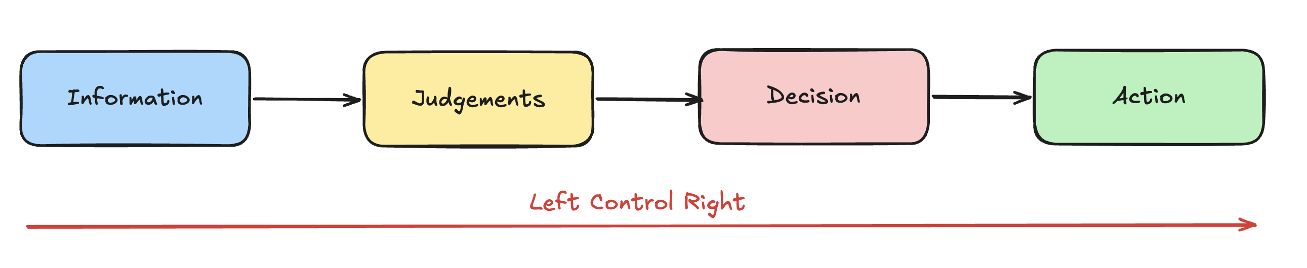
Note: only used when you need to have information of the action -> not judgment.
4.14. What are vector clocks and when would you use them over Lamport clocks?
Vector clocks assign a per-process counter in a vector of length N (one per process). On send, increment own counter and attach full vector. On receive, merge vectors element-wise by taking the max, then increment own counter. They capture the full causality structure: A happened-before B iff every element of V(A) is ≤ the corresponding element of V(B). Use vector clocks when you need to detect conflicts (concurrent writes) in a leaderless system. DynamoDB uses a variant to detect when two writes are concurrent and need client-side resolution.
4.15. What is a Hybrid Logical Clock (HLC) and why does CockroachDB use it instead of pure Lamport clocks?
HLCs combine physical time with a logical counter: HLC = (physical_time, logical_counter). On each event, advance to max(local HLC, message HLC), then increment logical counter only if physical times are equal. This preserves causality like Lamport clocks but keeps timestamps close to wall clock time, enabling time-based queries (“give me all events before 2pm”) and bounded clock skew assertions. CockroachDB uses HLCs so that transaction timestamps are meaningful calendar times while still ensuring causality across nodes without TrueTime hardware.
4.16. How does Google Spanner achieve external consistency using TrueTime?
TrueTime exposes time as an interval [earliest, latest] that bounds the true current time. Before committing a transaction, Spanner assigns a timestamp S = TT.now().latest, then performs commit wait: it blocks until TT.now().earliest > S. This guarantees that any transaction starting after this one observes a strictly later physical time, providing external consistency (linearizability across datacenters) without network round trips. The maximum wait is approximately 2ε where ε is the clock uncertainty bound (typically 3-7ms).